CS365:Homework 3

Submitted By

Pratap Bhanu Solanki Y9429

Problem A

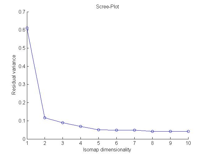
Here we can see the elbow of scree plot occurs at dimensionality 2. Hence dimensionality of this manifold is best explained at 2.

Problem B

Problem C

Variation of Theta1 at constant Theta2 = 90 degree

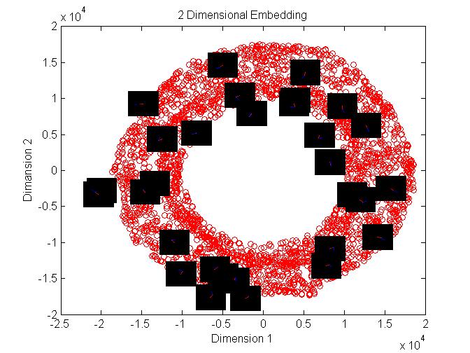
Here in the above figure we can see that Theta1 varies along the circumference of the Torous at a constant radius.

Problem D

Topology in 3D

It can be easily observed that the topology is Torous.

Problem E

Experimentation table

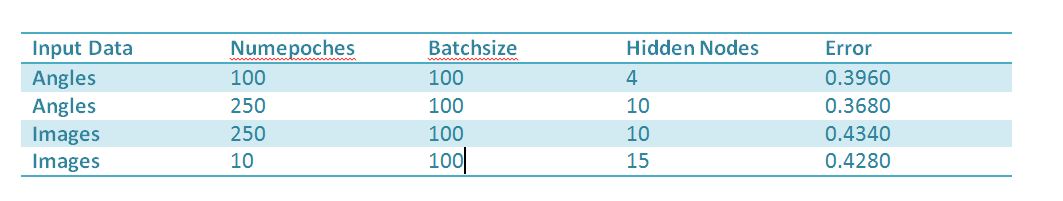
From the table we can see that Mean Square Error is less when input data is in form of angles. Though the useful information(2 Dimensional Angular Information) in both angles and images is same but since 'Angles' contains the information in precise format, it is taking less time to learn and also giving less error. Moreover The image data is represented in the form of 30000 dimensional vector so learning that efficiently is also a tough and tricky task.

Shortest Path between 00001.png and 00161.png

Problem F

Shortest path calculation while avoiding Obstacle 1

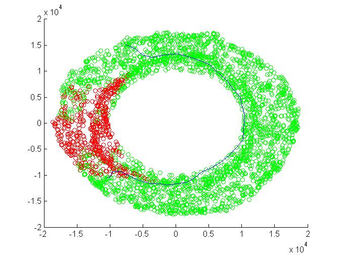
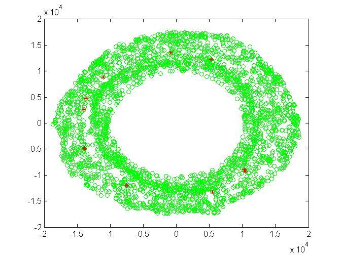
Here in the above figure green circles represents the configurations where Robot is not hitting the obstacle. The Red circles denotes the configurations when the arm is hitting/overlapping with the obstacle
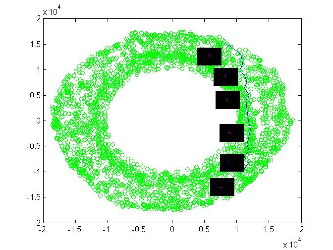
The blue curve denote the shortest path between nodes corresponding to image 00001.png and image 00161.png. The path is taking so long round because the direct path between the nodes does not exists. The obstacle is in the range of first link so the Torous is being fully sected at the area corresponding to obstacle.

Problem G

Shortest path calculation while avoiding Obstacle 2

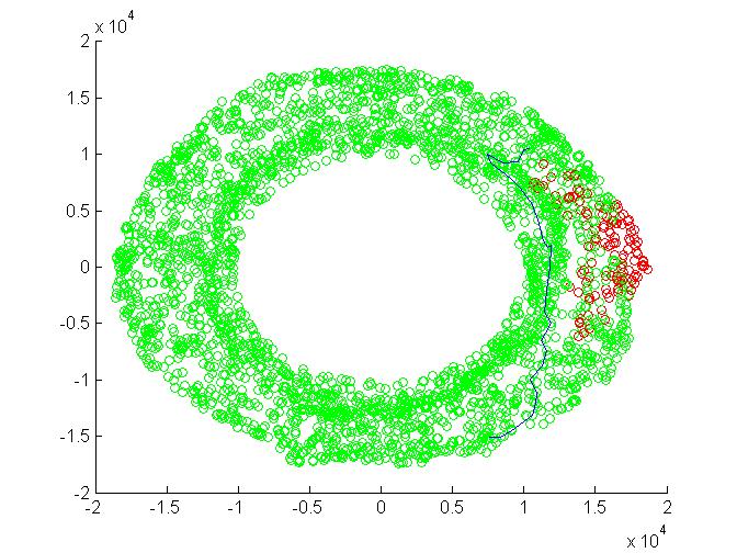
This part is similar to part F except the fact that here the torous is not fully sected at the area corresponding to obstacle. It is because the obstacle now is out of range of first link. Hence the shortest path observed seems to be direct path.