Artificial Intelligence CS365 - Homework 1
A : k-NN based classifier
Matlab code : File q1.m
Matlab code : File loadDigits.m
Remarks : Training Set 3000, Test Set 1000
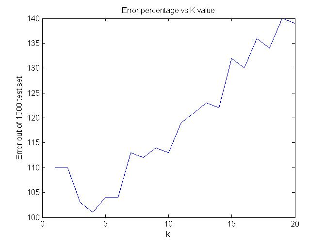 Observations about data set based on the graph :
Maximum Accuracy is obtained at k=4 only 101 wrong samples out of 1000
Observations about data set based on the graph :
Maximum Accuracy is obtained at k=4 only 101 wrong samples out of 1000
B : Manifold based modeling of MNIST digits
Isomap Brief :
Isomap solves the problem of Dimensionality redution.
In isomap geodesic distances are incorporated on a weighted graph with metric MDS(Multi-Dimensional Scaling). This is done to incorporate manifold structure in the resulting embedding.
Geodesic Distance accoring to Isomap : sum of edge weights along the shortest path between two nodes.
The particular Isomap algorithm used here learns the global geometry of dataset using local metric information.
Using Euclidean Distance
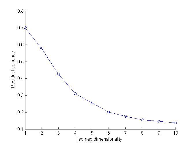
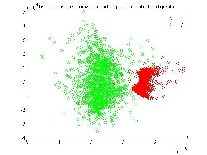
a. 1 and 7
Matlab code : File q21.m
Matlab code : File loadDigits17.m
Matlab code : File L2_distance.m
Matlab code : File Isomap17.m
Graphs :
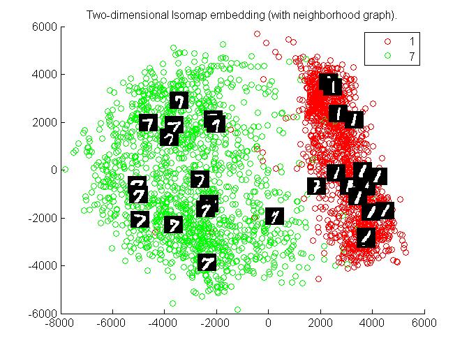
 Observations :
clusters of 1 and 7 are separate and can be identified easily. Hence for 1 and 7 this algorithm works very effectively.
Observations :
clusters of 1 and 7 are separate and can be identified easily. Hence for 1 and 7 this algorithm works very effectively.
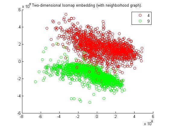
b. 4 and 9
Matlab code : File q22.m
Matlab code : File loadDigits29.m
Matlab code : File L2_distance.m
Matlab code : File Isomap29.m
Graphs :
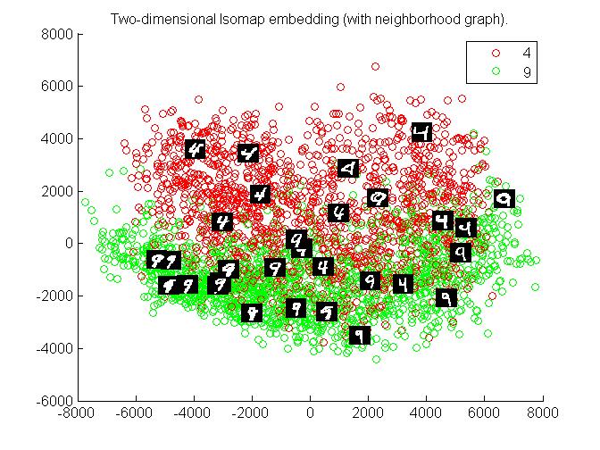
 Observations :
clusters of 4 and 9 are sort of mixed up in middle, hence can not be identified easily. Hence for 4 and 9 this algorithm is not very efficient.
Observations :
clusters of 4 and 9 are sort of mixed up in middle, hence can not be identified easily. Hence for 4 and 9 this algorithm is not very efficient.
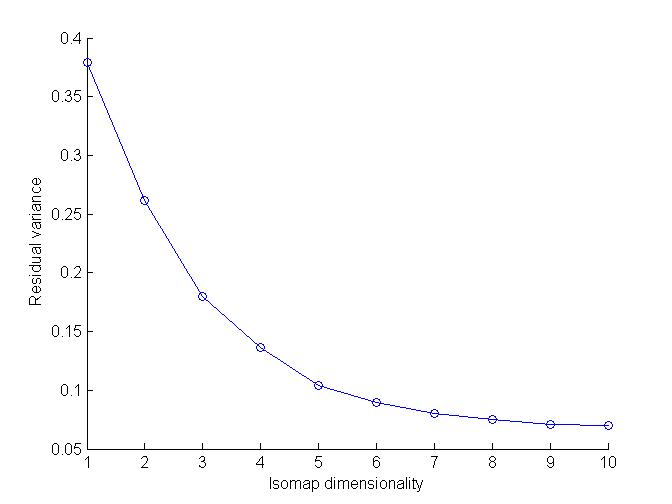
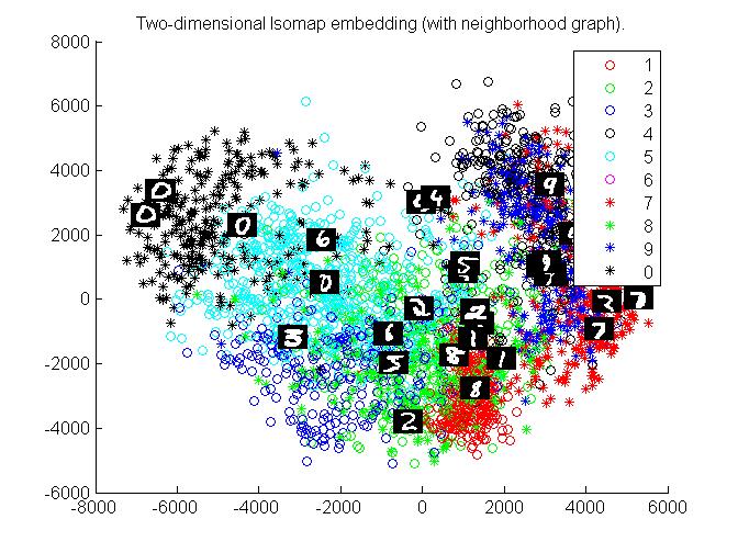
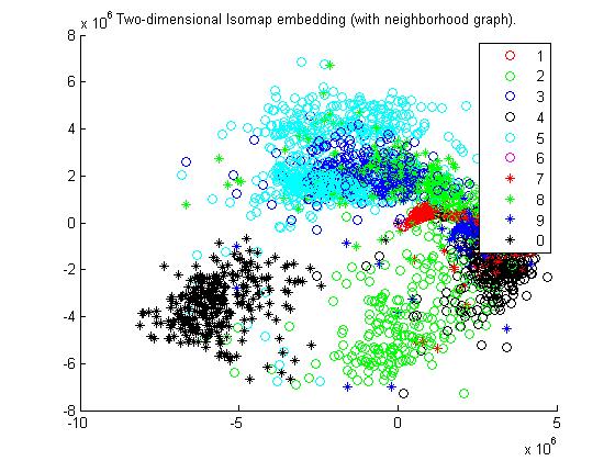
c. All the digits
Matlab code : File q23.m
Matlab code : File loadDigits.m
Matlab code : File L2_distance.m
Matlab code : File Isomapad.m
Graphs :
Extra Credit :
Shown in part (a),(b) and (c) above.
Using Tangent Distance
a. 1 and 7
Matlab code : File q21t.m
Matlab code : File loadDigits17.m
Matlab code : File tangent_d.m
Matlab code : File Isomap17.m
Graphs :
 Observations :
As from Graph, 1 and 7 can easily be separated. Hence this algorithm also works efficiently for 1 and 7.
Observations :
As from Graph, 1 and 7 can easily be separated. Hence this algorithm also works efficiently for 1 and 7.
b. 4 and 9
Matlab code : File q22t.m
Matlab code : File loadDigits29.m
Matlab code : File tangent_d.m
Matlab code : File Isomap29.m
Graphs :
 Observations :
4 and 9 are distinguishable more comfortably as compared to technique of Euclidean distance. Hence tangent distance works much better for 4 and 9.
Observations :
4 and 9 are distinguishable more comfortably as compared to technique of Euclidean distance. Hence tangent distance works much better for 4 and 9.
c. All the digits
Matlab code : File q23t.m
Matlab code : File loadDigits.m
Matlab code : File tangent_d.m
Matlab code : File Isomapad.m
Graphs :
 Observations :
Clusters of different digits are comparative more distinguishable to those of Euclidean ones.
Observations :
Clusters of different digits are comparative more distinguishable to those of Euclidean ones.
C. Deep Learning
Procedure of Experiment i.e. Working of Deep Architectures
DBNs are graphical models which learn to extract a deep hierarchial representation of training data.
Process is as follows : Put the initial input to train the first layer.Now, through output of first layer we can obtain input representation of 2nd layer. Now train the second layer and repeat the process for all layers. After fine tuning, result is obtained.
Here DBN sizes is architechture of network.
Observations while tweaking:
1). Increasing Learning rate upto 5-6 decreases error.
2). Increasing numepochs in DBN decreases error but increases time taken by code to run i.e. complexity
3). batchsize of dbn = 100 is optimal value. Decreasing/Increasing its value increases error.
4).Increasign alpha increases error.
5).Increasing numepochs in NN reduces error but increases complexity.
6). Decreasing Batchsize of NN, reduces error.
7). making Neural Network Architecture More complex i.e. increasign no. of layers dont have much impact on error rate. Increasign no. of neurons in one layer do impact significant effect.
Table
| DBN Sizes |
DBN Numepochs |
DBN batchsize |
DBN Momentum |
DBN Alpha |
NN learning rate |
NN numepochs |
NN batchsize |
ERROR percent |
| [100 100] |
1 |
100 |
0 |
1 |
1 |
1 |
100 |
8.91 |
| [100 100] |
1 |
100 |
0 |
1 |
2 |
1 |
100 |
7.56 |
| [100 100] |
1 |
100 |
0 |
1 |
3 |
1 |
100 |
6.94 |
| [100 100] |
1 |
100 |
0 |
1 |
4 |
1 |
100 |
6.52 |
| [100 100] |
1 |
100 |
0 |
1 |
5 |
1 |
100 |
6.13 |
| [100 100] |
1 |
100 |
0 |
1 |
3 |
2 |
100 |
5.72 |
| [100 100] |
1 |
100 |
0 |
1 |
3 |
4 |
100 |
4.48 |
| [100 100] |
1 |
100 |
0 |
1 |
3 |
6 |
100 |
4.13 |
| [100 100] |
1 |
100 |
0 |
1 |
3 |
10 |
100 |
3.69 |
| [100 100] |
1 |
100 |
0 |
1 |
3 |
10 |
50 |
3.35 |
| [100 100] |
1 |
100 |
0 |
1 |
3 |
15 |
50 |
3.02 |
| [100 100] |
5 |
100 |
0 |
1 |
3 |
15 |
50 |
2.81 |
| [100 100] |
15 |
100 |
0 |
1 |
3 |
15 |
50 |
2.61 |
| [100 100] |
5 |
50 |
0 |
1 |
3 |
15 |
50 |
3.08 |
| [100 100] |
5 |
100 |
0 |
2 |
3 |
15 |
50 |
3.44 |
| [100 100 100] |
5 |
100 |
0 |
1 |
3 |
15 |
50 |
3.03 |
| [200 200 200 200] |
5 |
100 |
0 |
1 |
4.5 |
30 |
50 |
2.27 |
| [100 100] |
5 |
100 |
0 |
1 |
4.5 |
30 |
50 |
2.12 |
| [100 100] |
5 |
100 |
0 |
1 |
4.5 |
30 |
50 |
2.27 |
| [100 100] |
1 |
200 |
0 |
1 |
1 |
1 |
100 |
9.95 |
| [300 300 300 300] |
5 |
100 |
0 |
1 |
5 |
15 |
20 |
2.68 |
| [200 200 200 200] |
5 |
100 |
0 |
1 |
4.5 |
15 |
20 |
2.82 |
| [300 300] |
5 |
100 |
0 |
1 |
4.5 |
15 |
20 |
2.04 |
| [400 400] |
8 |
100 |
0 |
1 |
4.5 |
20 |
10 |
2.00 |
After Tweaking, I was able to achieve a minimum of 2% error using parameters specified in above table.