Part A. Residual Variance v/s k

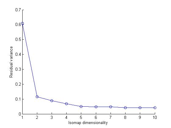
Error rate droops down significantly for k=2 nearest neighbours. After that as the value of 'k' increases, the classifier function matches the sample image with more and more neighbours, which does not affect much. As can be seen that the decrease in variance for higher values of 'k' is insignificant w.r.t. the previous decreament.

Part B

Part C

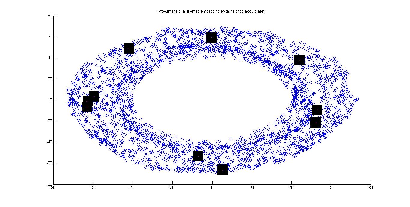
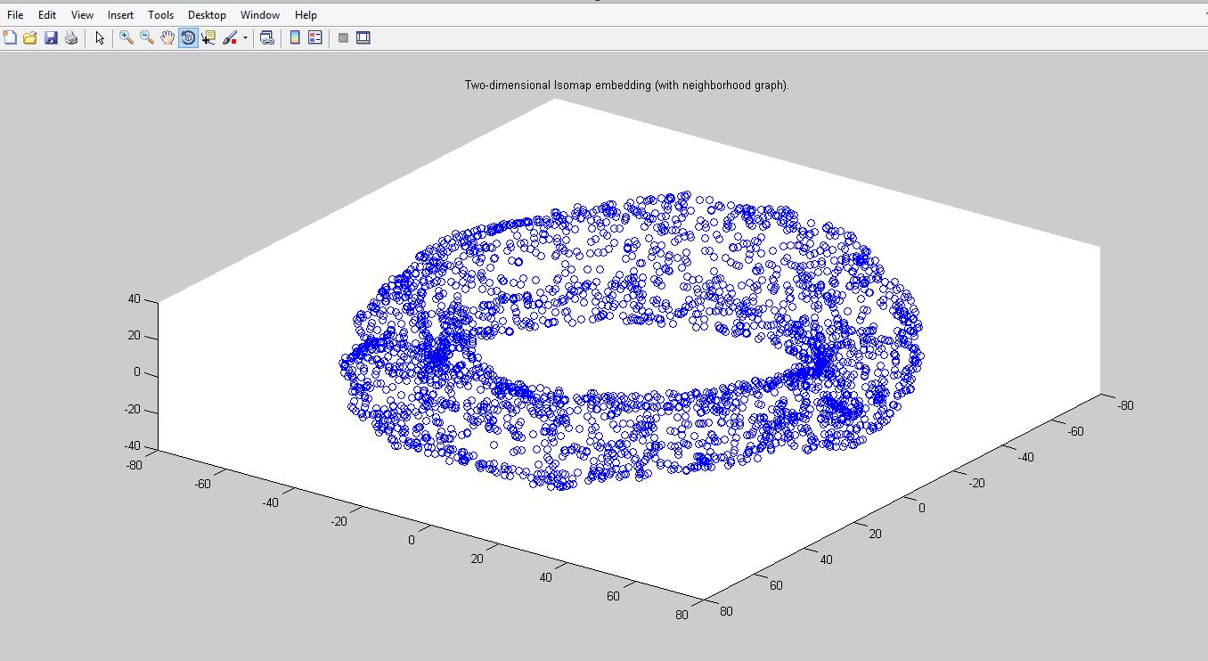
As in the images, we can see that both theta1 and theta2 are measured considering clockwise measured angles as positive.
If we see in the 3D embedding, we can conclude that for a particular theta1, the values of theta2 vary along a ring on the toroid, with the value of theta2 = 0 lying on the outermost equitorial point whereas +pi and -pi lie on the innermost equatorial points.
On the 2D isomap, theta2 varies along a straight line for a particular theta1. The variation of theta2 goes on as => 0 at the outermost point, then +(pi/2) and -(pi/2) lying at the centre and +pi and -pi on the innermost point.

Part D

Part E

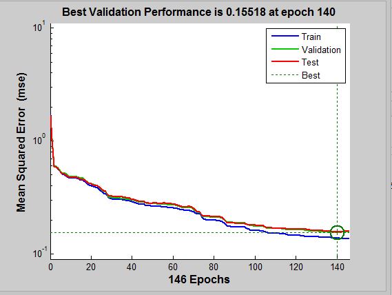
The performance plot when neural network was trained by angles i.e.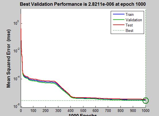 All other plots can be downloaded by clicking here
The performance plot when neural network was trained directly by images All other plots such as error histogram, training state etc. can be downloaded by clicking here

The path planned isomap of the data with no object present.

Part F

The 2D isomap without the images in which arm hits the object in the first location.
The plot also shows the path in blue lining.

Part G

The 2D isomap without the images in which arm hits the object in the second location. The plot also shows the path in blue lining.

Here we can see that unlike part F, all values of theta1 are possible, but for certain values of theta1, some valued of theta2 are not allowed. This happens because of the change in location of the object, which enables arm 1 to rotate freely at any angle in this case, but with some constraints on theta2 for specific values of theta1.