Salman Mohammad, 10630
HW3
Codes are available here.
A. Manifold Learning

The residual variance has the steepest decline at dimensionality = 2. So the dimensionality of this manifold can be best explained at 2.
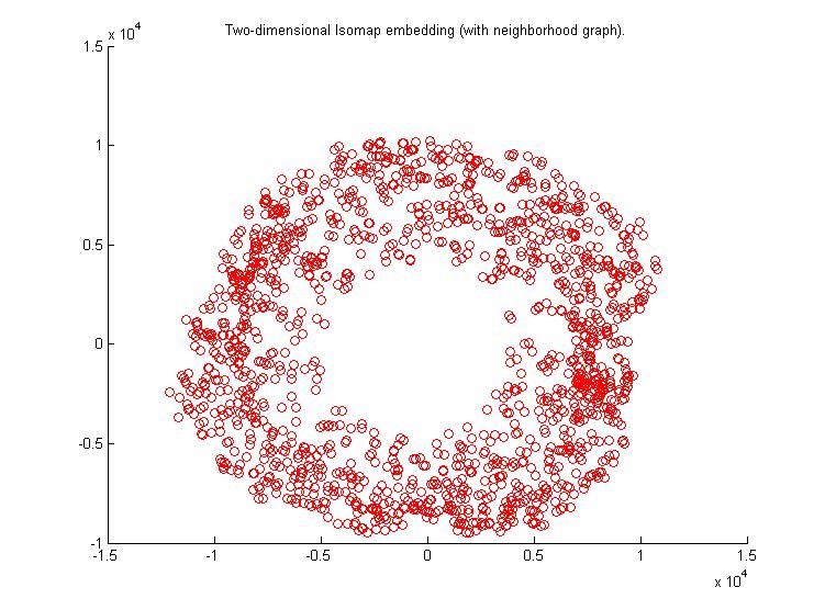
B. 2 Dimension Embedding

C. Variation of Theta1 and Theta2
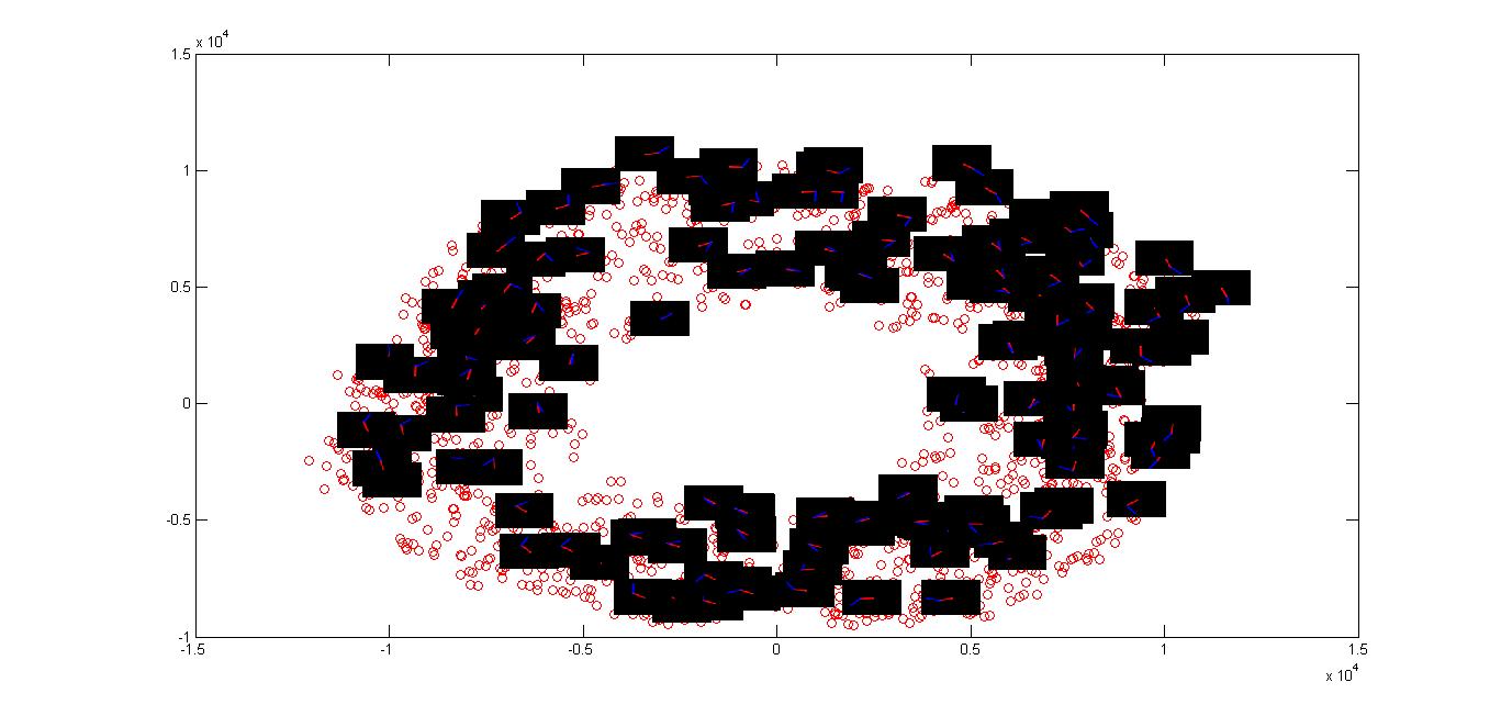
From the above image, we can see that as we move around the graph, Theta1 varies from 0 to 360 degrees. The map is able to capture the topology of the robot motion correctly.

When we zoom into a particular area, we can clearly see that in this region Theta1 is almost constant while Theta2 varies from 0 to 360 degrees.
D. Embedding in 3-D
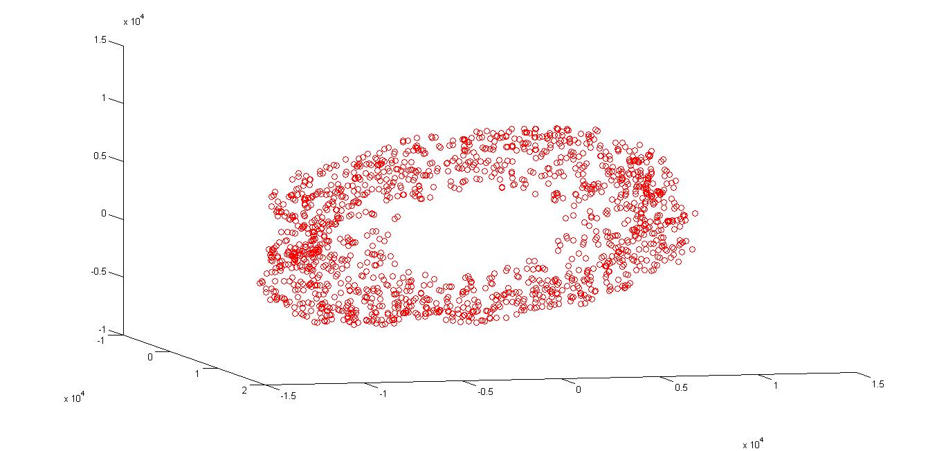
The topology is clearly a toroid.
E. Mapping and path planning
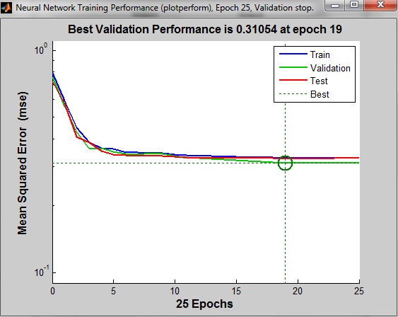
The map converges very quickly when we use . But if we try to model using the whole image, we run out of memory.
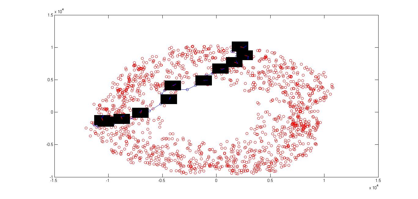
The path from image 1 to image 161 is shown above.
F. Obstacle avoidance for Obs1

G. Obstacle avoidance for Obs2

We see that in (F), the graph is not connected and so the robot will have to go around the map while in (G), there is a path available and the motion is more efficient. This is because, now the obstacle obstructs less number of configurations than before.