Recent advancement in DBNs have showed that it is possible to learn multiple layers of non-linear features without actually
using labelled data. Object recognition is one of the prominent challenges of artificial intelligence these days and and DBNs on
account of their unsupervised feature learning have contributed a lot in this field. Greedy layerwise training is performed i.e training
is done for one layer at a time as "Restricted Boltzman Machine" using "Contrastive Divergence". Fine tuning of the net is
done using supervised backpropagation after pretraining.
=>Restricted Boltzman Machine: An invariant of Boltzman Machine, with the restriction that each connection must
be between a hidden unit and a visible unit, unlike recurrent network (having connections among hidden units also). Its a kind of model which
is generative in nature and tries to learn probability distribution over its set of inputs[1][2].
=>Contrastive Divergence: It is one of the methods for trainig RBNs which is also fast enough. We propose a
probability distribution and try to fit the input data to that probability distribution by using many cycles of Markov Chain Monte Carlo
sampling. Since using many cycles of MCMC sampling is time consuming, we use few cycles of sampling in order to compute approximate
gradient instead of computing accurate gradient. The intution behind this is that after a few iterations data will have moved from the target
distribution towards proposed distribution[1][2][3].
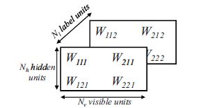
Till now DBNs only comprises of two types of observed units i.e one for the label of the object and one for the pneultimate feature vector irrespective of what is happening at the hidden level(hidden layer). This paper presented a Third-Order RBM as the top level model in which a joint distribution is moddled taking hidden unit also into consideration.The figure below presents a rough idea of initial and present approach.

In this way the parameters form a 3D tensor instead of a matrix as in earlier case.
An energy function is defined for the model which is given by

where W is a scaleable parameter. And the probability of full configuration is given by the following equation, where Z represents the partition function.

Defining label vector as a discrete random variable having K states represented as 1-of-K encoding, it is observed that
k-th component of label is if "1", then k-th slice of the tensor defines our energy function.
So we infer that the distribution that we are trying to model is P(l|v) for classification purpose and P(v,l|h) and
P(h|v,l) for learning based on Contrastive Divergence. Once l is observed the model reduces back to an RBM with parameters as
k-th slice of 3D tensor. The whole computation takes place in O(NvNhNl)
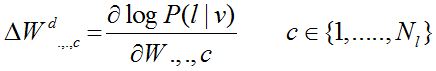
Contrastive Divergence learning is bascically formulated for bipartite architectured RBM as maximum likelihood learning is intractable. In this paper CD learning is extended for third order RBM also. Maximum likelihood gradient is computed by MCMC algorithm till the sampling chain reaches equilibrium. However, CD learning uses only three half steps of this chain initialized from a training data instead of randomly initializing.
The NORB Database consisted of five objects namely animals, humans,planes, trucks, and cars. Normalized version of the data base has been used. Each training example is a stereo pair of gray-scale images, size: 96x96.Based on the above explained algorithm different models are built like shallow models and deep models.It is obvious that deep model must perform better than shallow model. Introducing even one pre-trained layer, trained greedily, decreased the error rate a lot as compared to shallow model. It has been observed that third order RBM outperformed standard RBM top level model having same number of hidden units. Comparing "hybrid learning rule" and "CD" learning rule for the top level RBN, there is not much difference cited between the two error rates, however, hybrid is better.
The two main points to conclude are:
1) Using generative model in object recognition gives a lot better result because it produces a representation of the input image which gives
more acurate result as compared to raw pixels.
2) Including P(v|l) in the learning rule along with P(l|v) fro trainig the top level model improved the performace of the
classification task.
[1] Wikipedia
[2] www.deeplearning.net
[3] http://www.robots.ox.ac.uk/~ojw/files/NotesOnCD.pdf
[4] Images are taken from the review paper itself.