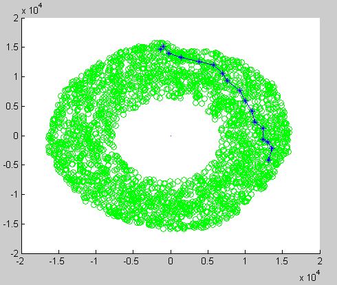
The figures below show the 2D Isomap Plot and residual variation with dimension. As evident from the residual graph, we can see that maxium residual variation is corresponding to dimension '2'. From this we infer that dimensionality of the manifold is best explained at '2'.

Following figure shows the variation of Theta1 over the manifold.
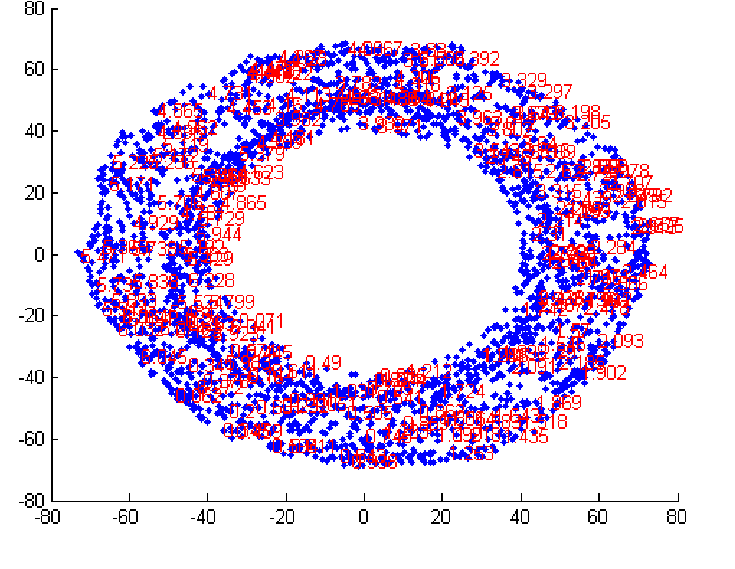 As in the images, we can see that both theta1 and theta2 are measured considering clockwise measured angles as positive. If we see in the 3D embedding, we can conclude that for a particular theta1, the values of theta2
vary along a ring on the toroid, with the value of theta2 = 0 lying on the outermost equitorial point whereas +pi and -pi lie on the innermost equatorial points.
On the 2D isomap, theta2 varies along a straight line for a particular theta1. The variation of theta2 goes on as : 0 at the outermost point, then +(pi/2) and -(pi/2) lying at the centre and +pi and -pi on the innermost point.
As in the images, we can see that both theta1 and theta2 are measured considering clockwise measured angles as positive. If we see in the 3D embedding, we can conclude that for a particular theta1, the values of theta2
vary along a ring on the toroid, with the value of theta2 = 0 lying on the outermost equitorial point whereas +pi and -pi lie on the innermost equatorial points.
On the 2D isomap, theta2 varies along a straight line for a particular theta1. The variation of theta2 goes on as : 0 at the outermost point, then +(pi/2) and -(pi/2) lying at the centre and +pi and -pi on the innermost point.
From the 3 Dimensional plot we can see that the topology followed by the robotics arm is of a "TOROID".

As evident from the following two figures, learning the desired mapping is faster in case we learn it from 2D Isomap manifold as it converges faster. But when we train with images directly, the number of epochs required are much larger(172 here) as compared to previous method(only 6) because we are working in a very high dimension and number of training examles is also less with respect to the nubber of features. The first graph correspond to training from Isomap manifod. The second graph correspond to training directly from images.


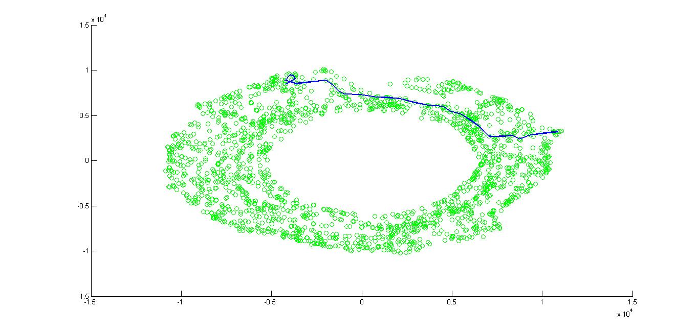
Here we can see that unlike part F, all values of theta1 are possible, but for certain values of theta1, some valued of theta2 are not allowed. This happens because of the change in location of the object, which enables arm 1 to rotate freely at any angle in this case, but with some constraints on theta2 for specific values of theta1.