Anant Raj 10086
Link for all the codes is given below.
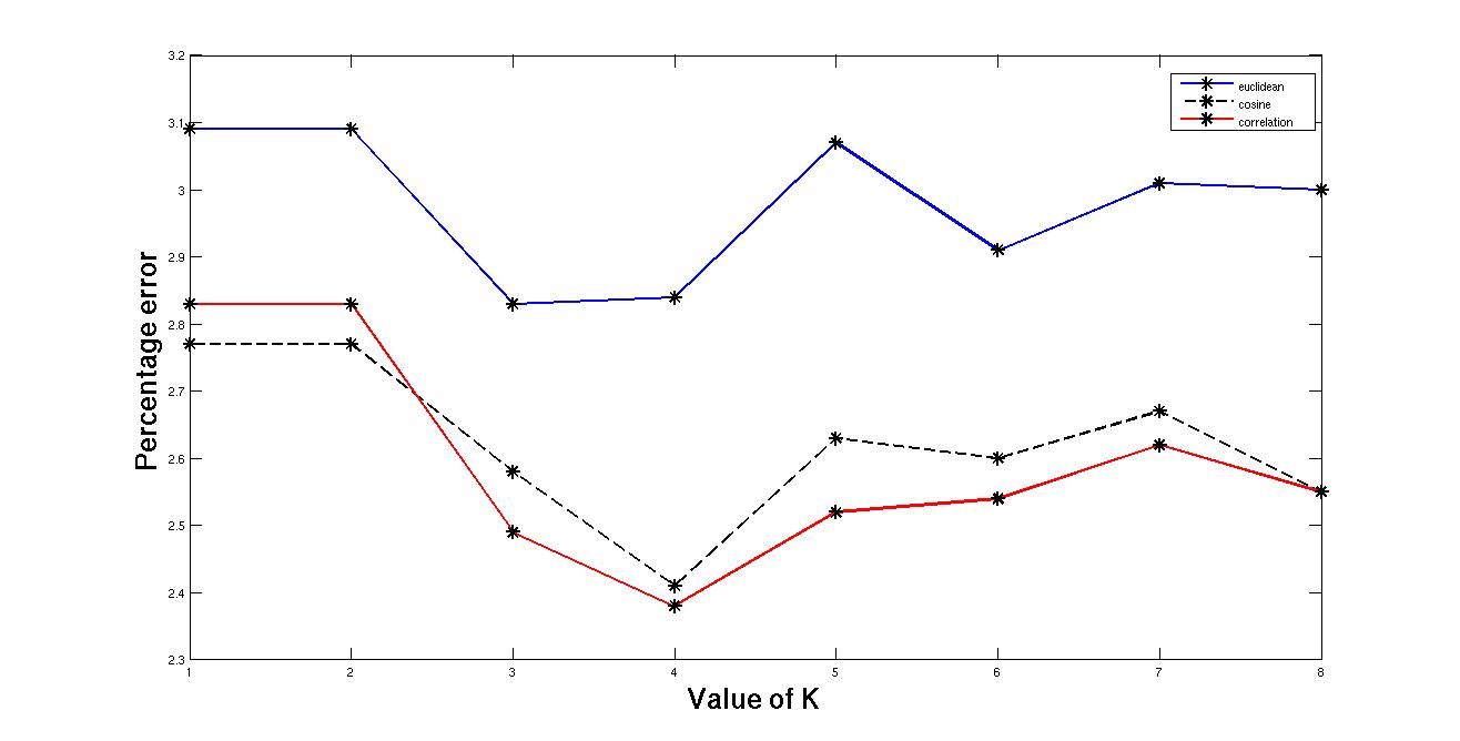
The above result is obtained after ruuning the knn classifier on tesst images of 10000 given training images of 60000. The best result is obtained for correlationl distance for the value of k = 4. This matlab funtion has been also run on lower dataset taking 10000 images as train image and testing on 3000 image. Then best result is found for K= 3. The reason for that is as the no. of images incleases the cluster is becoming dense and so more neighbour can be found of its own group. As the size of K is increased then the neighbours also come from different clusters. That's why percentage error increases after a certain value of K Running for such a large image on K is expensive in terms of time because every time the distance is calculated between new test image and each and every train image. This is a lazy form of learning.
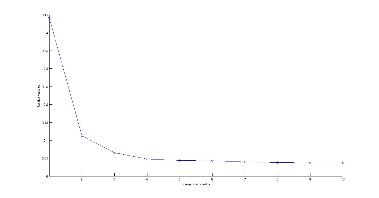
Isomap is a very effective non linear dimensional reduction technique. This is extended form of multidimensional scaling. But in place of euclidean matrix as in multidimensional scaling the distance along the manifold is calulated along using the shortest path in graph algorithm and the corresponding matrix is used as mentioned in one of the pioneer paper of non linear dimensionality reduction(Joshua B. Tenenbaum and Vin de Silva and John C. Langford, A Global Geometric Framework for Nonlinear Dimensionality Reduction).
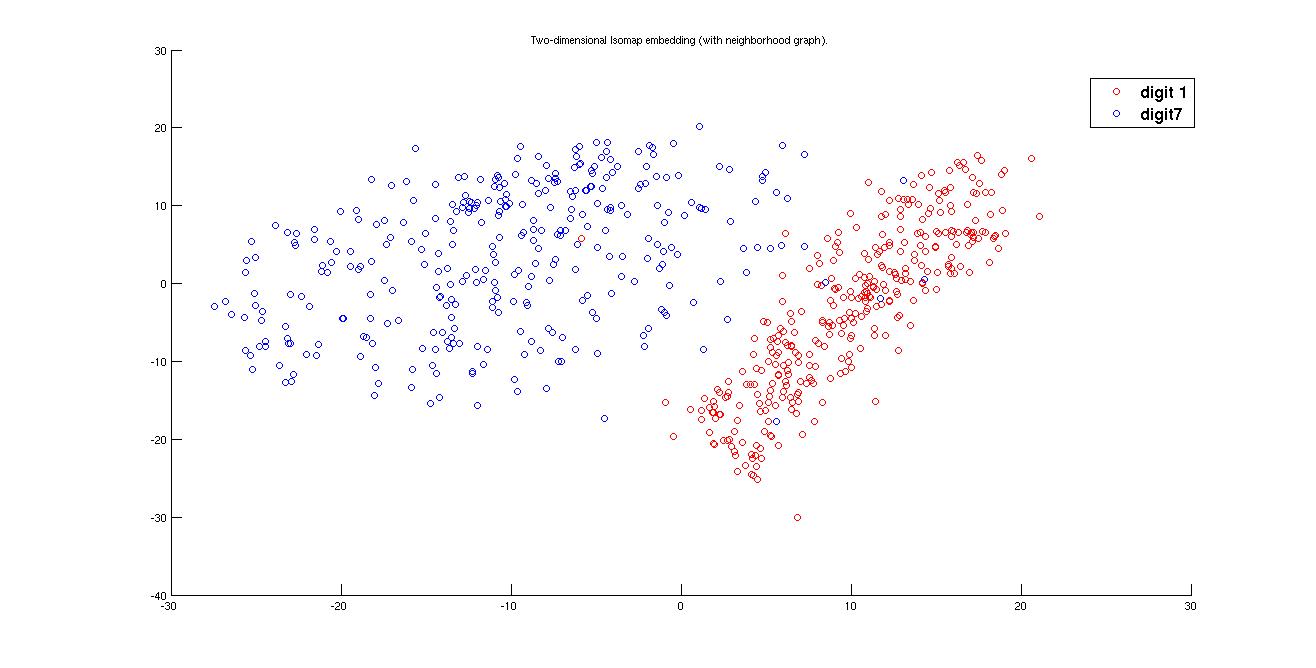
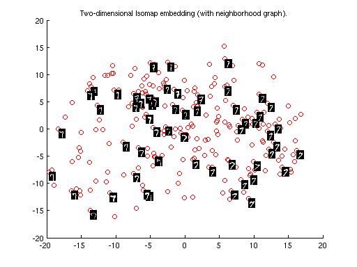
(i) Cluster plot for Digits '1' and '7' -
(a) Using Euclidean Distance
(b) Using Tangent distance
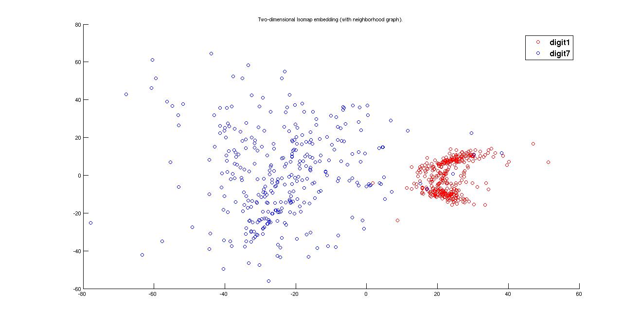
Here we see that cluster of 1 is spread all over the plane because writing 1 and 7 are not of much difference. 1 can be written in may ways and in some case it may look like 7 but there is not much choice to write 7 we get more dense cluster of 7. Also the best clustering is got in the case of tangent distance matrix because euclidean is a very general approach to find the distance matrix, it does not consider the case of variance or the direction of spread of data.
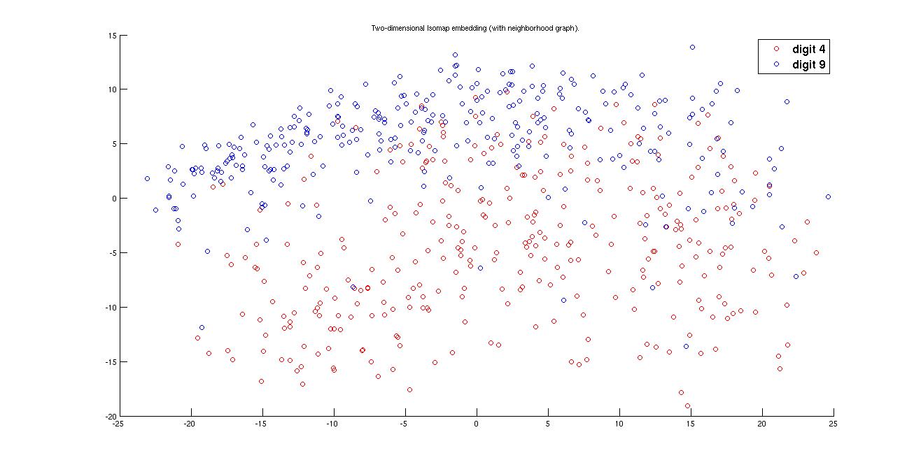
(ii) Cluster plot for Digits '4' and '9' -
(a) Using Euclidean distance
(a) Using Tangent distance
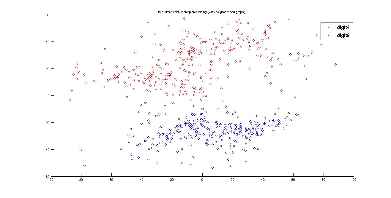
Here it can be observed that in case of Euclidean distance matrix the cluster of 4 and 9 is intermixed because of the well deserved reason. But in the case of tangent distance it seperates both of the two cluster upto a ggod mark.
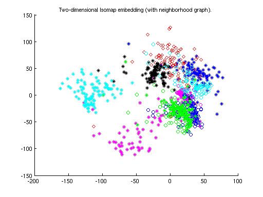
(iii) Cluster plot for All the Digits on 1000 dataponts. -
(a) Using Euclidean Distance matrix

(b)Using Tangent Distance matrix
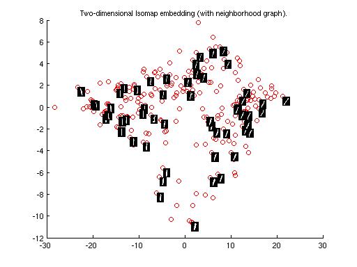
Now to show the variation of how the cluster's spread varies depending on the different thickness of digits and different style of writing some pictures are given with the digits displayed on them
Cluster plot for Digit "1" -
Cluster plot for Digit "4" -
Cluster plot for Digit "9" -
So it can be observed in the figure that when the tilt of digit of is increased towards right then it's cluster shift towards 7 and same in the other case also.
Deep architecture is an unsupervised form of learning. It work on the principal of generating a model of the given datasets. The advantage of using this model over neural network archtecture is that the training procedure is significantly fast in this case. When neural network architecture is used than after multiple layer the effect of back propagated error is not reflected effectively. So what we do try to do in the initial layer is to train the layer such that it reflects the input itself. So effectively the input data points are left open and each and every hidden unit tries to learn some good features independent of features learn by other hidden units out of the data points. Effectively it can be said that each hidden unit is representive of some unique features of the input data points. This process is carried forward to the multiple layers by taking the previous learn features as input and reflecting itself as the output. So ultimately some unique features are learnt in relatively low dimensional space which gives the better result on applying classifiers on it.
Here results are shown for some cases. Though the taken architecture is not correct for which my best result is coming out. Feature vectore should be compressed in every next layer. But when initially I took the Architecture structure of [250 100 50]
then the error rate is coming out 12.05. So I went for choosing the architecture such that firstly I compressed the feature vecture and then spread it out. (i)(Best Case)