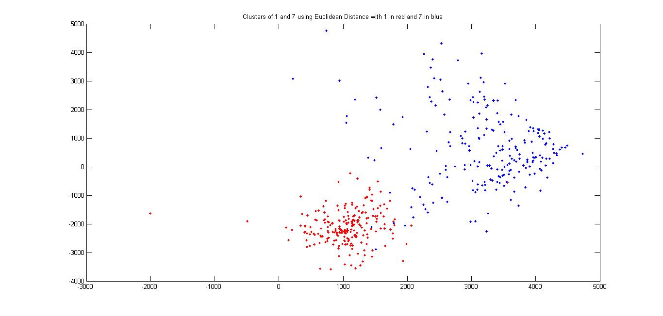
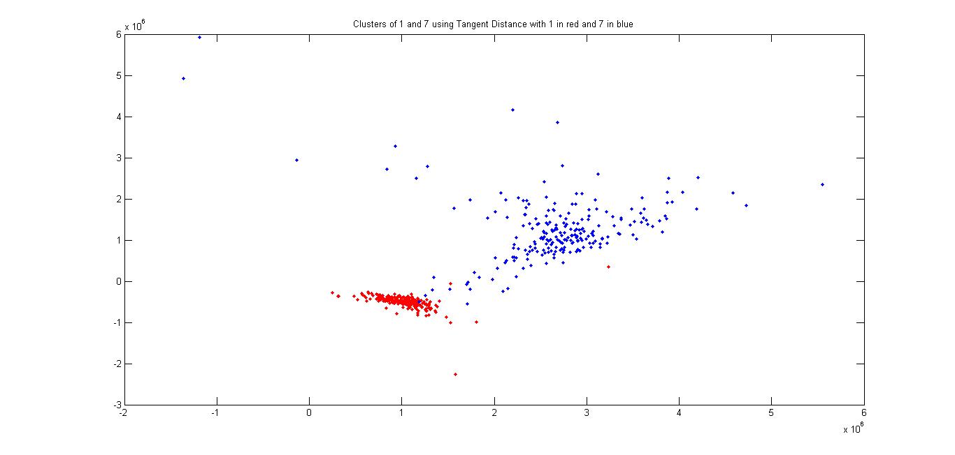
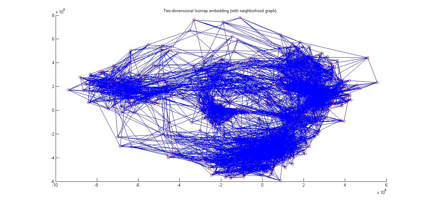
a. Clusters for digits 1 in red color and 7 in blue color.
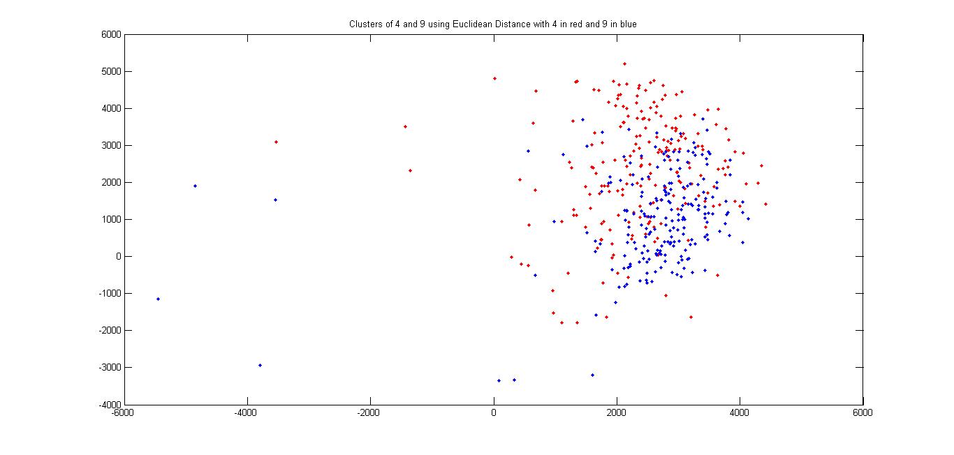
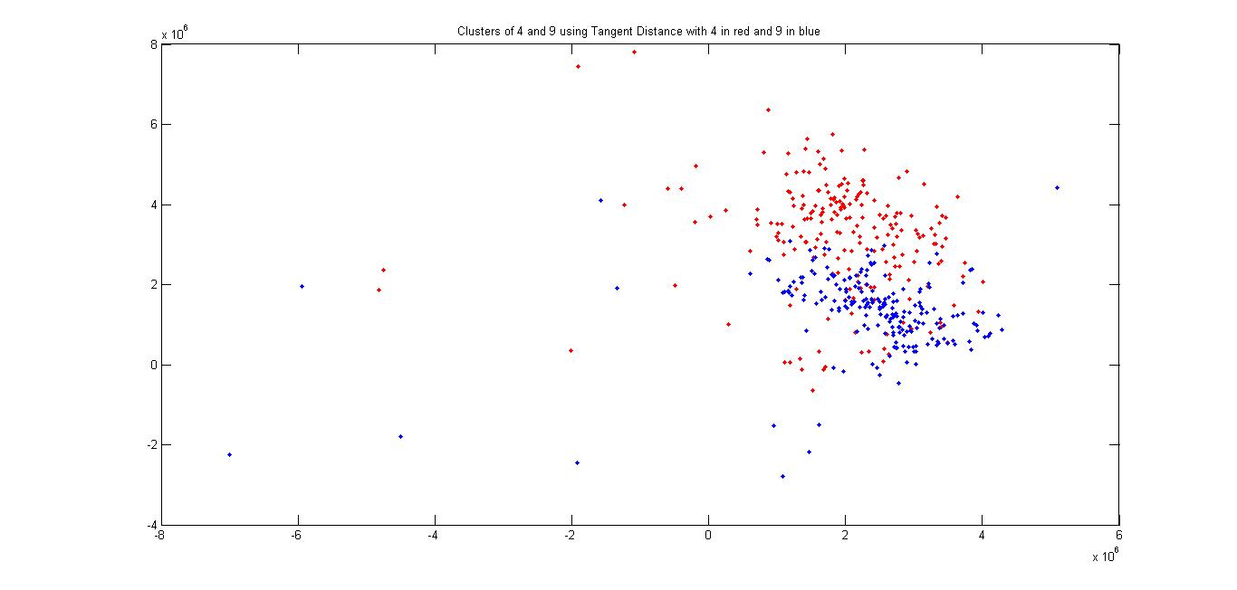
b. Clusters for digits 4 in red color and 9 in blue color.
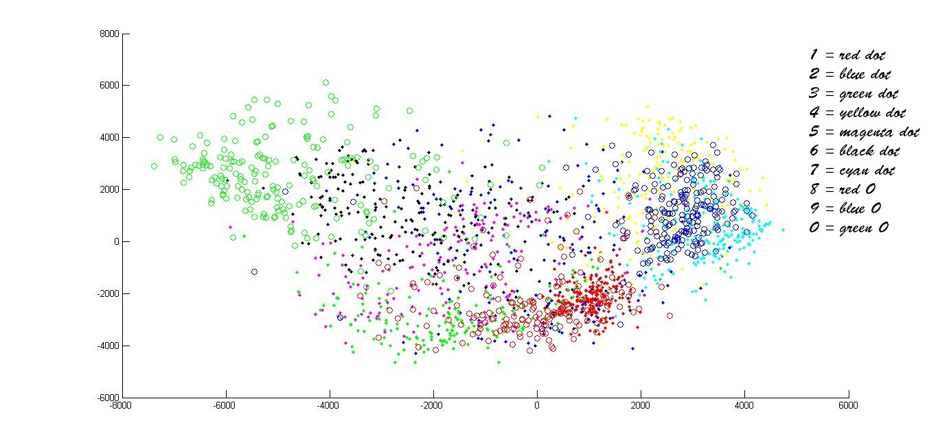
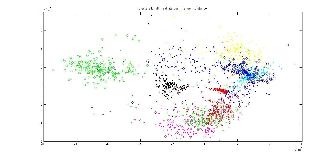
c. All the Digits.
a. Clusters for digits 1 in red color and 7 in blue color.
a. Clusters for digits 4 in red color and 9 in blue color.
c. All the Digits
The explanations regarding the codes can be found in the Readme.txt file in the folder Codes.zip
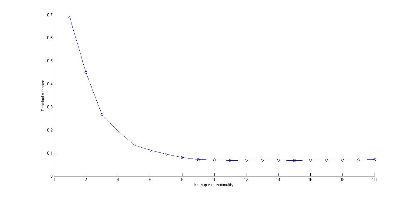
PART A: The Aldebaran Nao
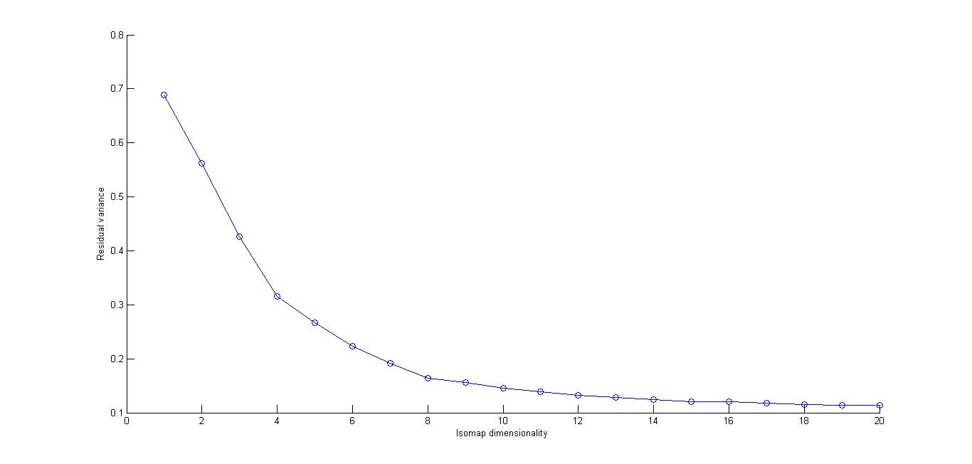
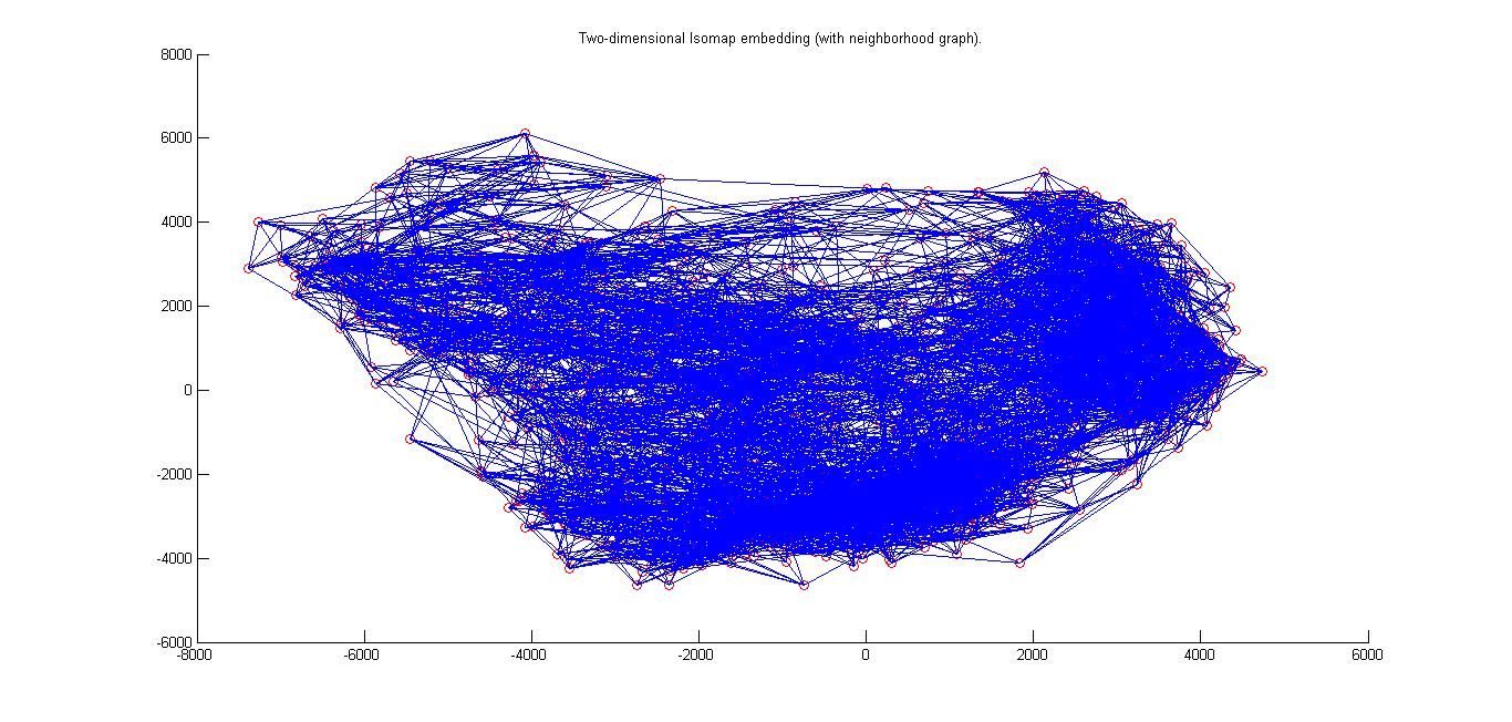
The value of K for nearest neighbours in isomap algorithm was taken to be 12 as it seemed to be giving the least residual error
Dimensionality: The most likely dimensionality of this data as suggested by the residual error curves is 2 as the elbow(as termed in the paper) of the curve
lies at dimension 2. That is the variation in residual error reduces significantly as one moves from 2 to higher dimensions.
Explanation: This is quite as expected as in the given set of images the robot can be observed to be using only 2 degrees of freedom, one of the
shoulder and the other at the elbow and the rest of the part remains practically constant in all the images.
Thus, in this case, isomap has been able to successfully bring down the dimensionality of the data to not only a managable number, but in all
probability to 2 meaningful dimensions representing the actual physical degrees of freedom.
PART B: The Robot Arms
The value of K for nearest neighbours in isomap algorithm was taken to be 7 as it seemed to be giving the least residual error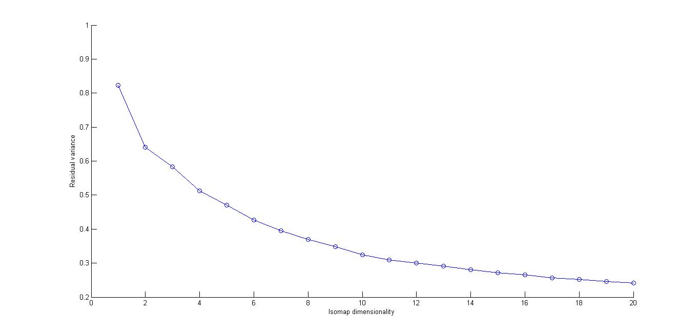
Dimensionality: It is difficult to single out one likely number in the curve as an elbow occurs at 2, but then again at 4 and then at 10.
Still,the most likely dimensionality of this data as suggested by the residual error curves seems to be 4 as the variation in residual error reduces
significantly as one moves from 4 to higher dimensions.
Explanation: This can be explained by the fact that the robots have 4 degrees of freedom as suggested in the problem, and verified (though not very
strongly) by the residual error curve. In this case also, more or less the dimensionality has been brought down to practically meaningful DOFs.
PART C: The Angles
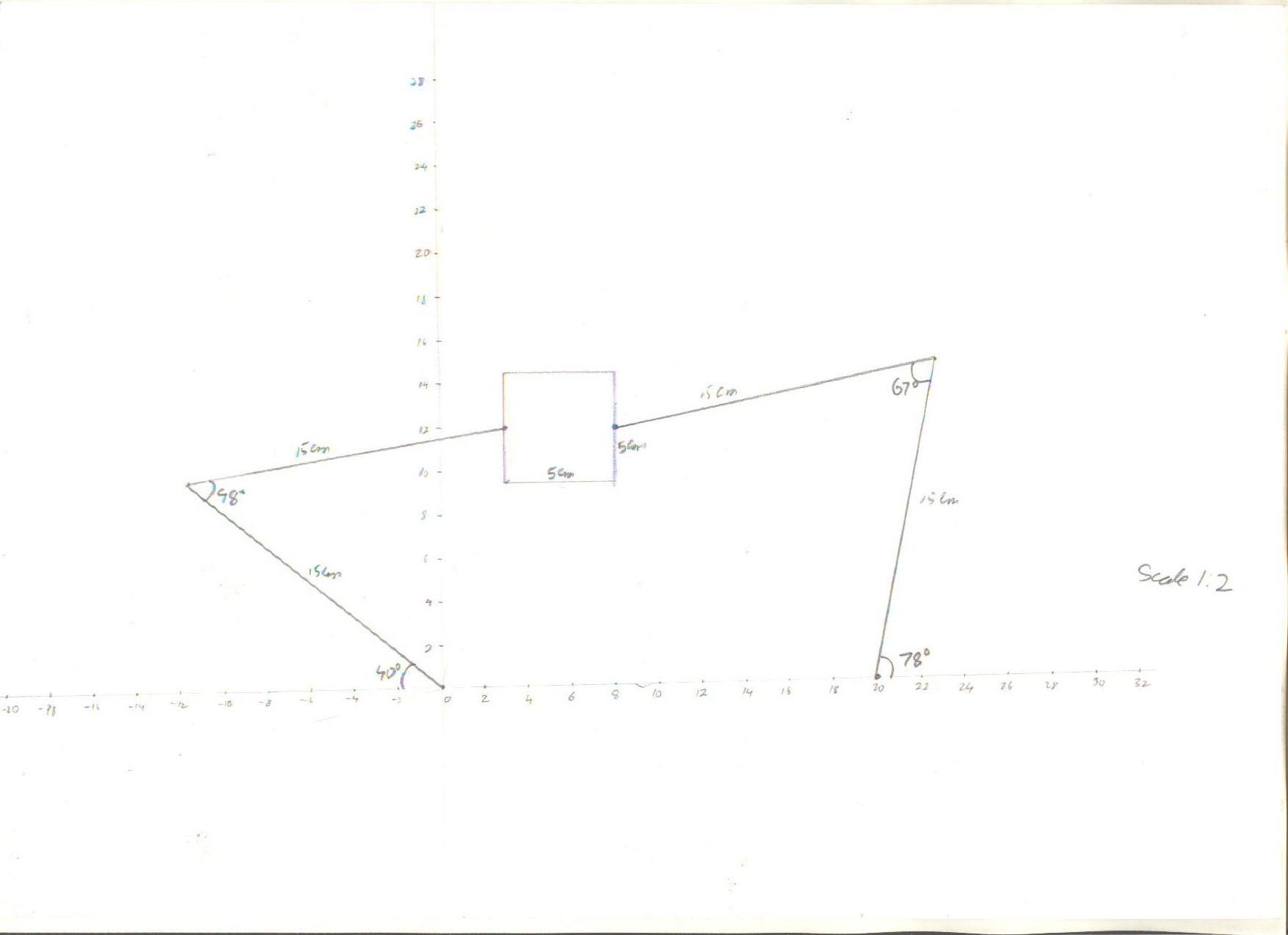
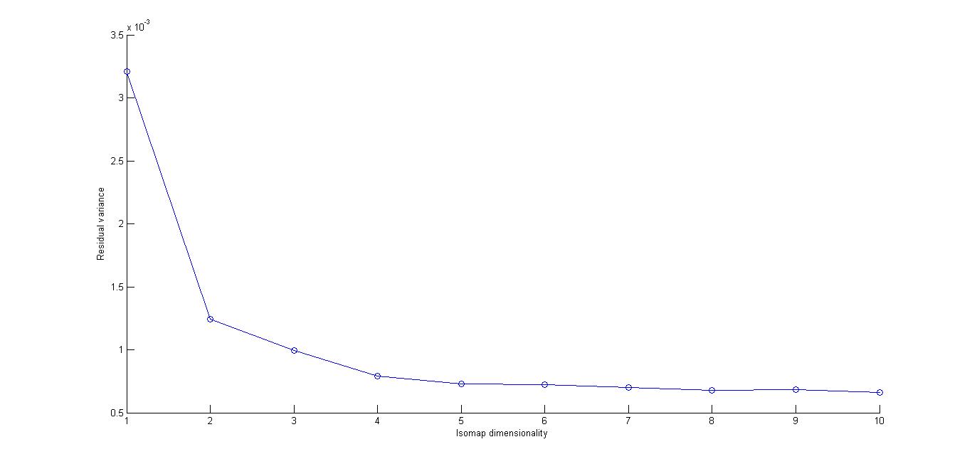
PART D: The Box
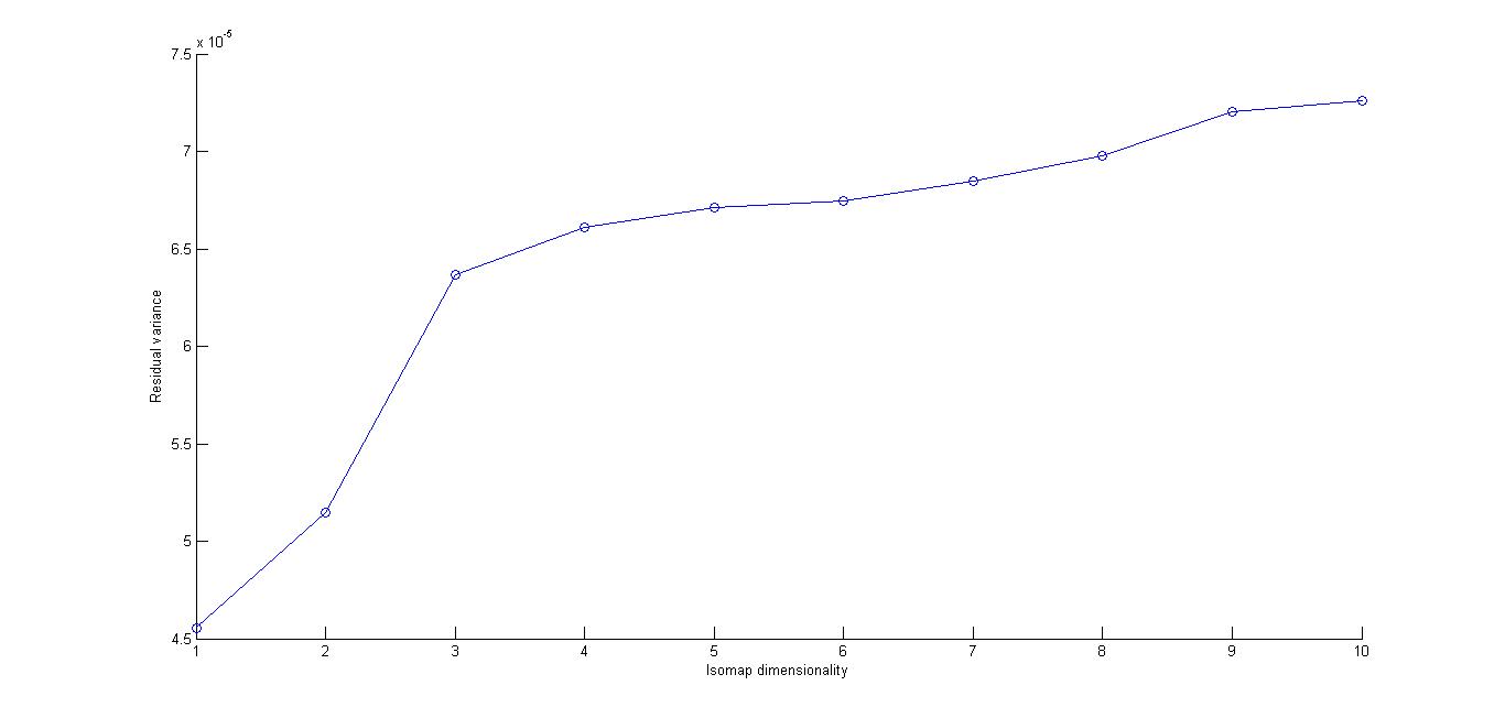
The value of K for nearest neighbours in isomap algorithm was taken to be 3 as it seemed to be giving the least residual error
Dimensionality: The most likely dimensionality suggested by the curve is 1.
Explanation: This can be explained by the fact that the complete change in the configuration depends only on the position(coordinates) of the box and
practically nothig else. In the given image sequence the box only moves horizontally , hence 1 degree of freedom as rightly suggested by the isomap curve.
For questions B1,B2 and B4, We have taken a different approach then suggested. LodeImageData.m and then L2_distance.m essentially resize
the image down to a 100x100 image and then compute the Distance Matrix D. Instead, we have written a function D_gen.m, which generates the D matrix taking
from the images without resizing them. This function takes 1 image at a time and computes the row in Distance matrix D corresponding to that image, i.e.
it calculates the distance of 1 sample from all other samples in one iteration of the outer loop. this procedure has the advantage of giving more accuracy because
it is considering all pixels, but it takes much more time (time complexity increased to save space, otherwise it runs out of memory).
As this procedure takes a long time (around half an hour), we decided to do it once for all the 3 parts B1,B2 and B4 and store the corresponding Distance
matrices in
nao_data.mat
box_random.mat
box1.mat
respectively. The files that were generated by us have been put in the same folder 'Codes'.
In the scripts for these parts, these files are loaded, and used directly.
Ankit Bhutani : A1 and A2, B1 and B2
Shubhdeep kochhar : A1 and A2, B3 and B4
nearly all the problems were done together