Decoupled Planning

This means to first plan the path of each robot more or less independently of each other, then consider the interactions among the paths. This method reduces the computational complexity of a multi-robot path-planning problem, because:

Centralized Planning is exponential in m = Sm_i i=1 to p

Decoupled Planning is exponential in max _iÎ[1,p] {m_i}

Demerit: Loss of completeness: The decoupled approach may fail to generate the path even if one exists and can be generated from Centralized Planning.

Prioritized Planning

Considering the motions of one robot at a time:

· The path of A₁ is planned in C, not in CT₁, ignoring all the other robots.

· Then the path of A_i is generated in the configuration-time space CT_i of A_i, avoiding collision with both: the obstacles B_j (j=1 to q) and the robots A₁ to A_i-1.

Hence the motion of A_i is planned as if that particular robot is moving among q stationary and i-1 moving obstacles.

· An arbitrary velocity is assigned to A₁, which does not have any bearing upon the final joint-path generated. This velocity merely determines the scale factor along the time axis of the C-spaces of the other robots.

The ordering on the robots requires a priority to be assigned to each robot:

· Random distribution

· Higher priority to the robots bigger in size.

· Assigning priorities by attempting to maximize the number of robots, which can reach their respective goals by moving along a straight line from their respective starting positions.

Path Coordination

It is based on a scheduling technique for dealing with limited resources (here space is shared). It consists of first generating the free path for each of the two robots (independently of the presence of the other robot), and then coordinating the two paths for avoiding collisions.

The approach works only for a 2-robot system.

Assume,

t₁ : s₁ Î [0,1] à t₁(s₁) Î C_1,free

t₂ : s₂ Î [0,1] à t₂(s₂) Î C_2,free are the two free paths generated.

C_1,free (resp C_2,free) denotes the free space in the configuration space of A₁( resp A₂) obtained by ignoring the other robot. Now we construct what is called the Coordination Diagram:

>> Construct something called s₁s₂ space [0,1]*[0,1]. Any continuous path in this space connecting (0,0) to (1,1) is called a schedule and determines the simultaneous traversal of the two paths by the respective robots.

eg (0,0) --> (1,0) --> (1,1) ==>A₁ completely travels t₁, and then A₂ completely travels t₂.

>> Now we define the obstacle region in the s₁s₂ space as the set of pairs (s₁,s₂) st

A₁(t₁(s₁)) Ç A₂(t₂(s₂)) ¹ f

>> Construct a free schedule in this coordination diagram that does not travel through this obstacle region.

Thus we have constrained the path of A = {A₁,A₂} in the composite configuration space of C₁*C₂ to lie in the intersection of the two subspaces whose projections into C₁ and C₂ are t₁ and t₂ respectively.

< figure 1 >

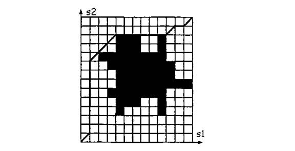
Subdivide each path t_i (i=1 or 2) into a sequence of w_i path segments determined by the intervals d_i,ki = [s_i,ki , s_i,ki+1], with k_i = 0, …, (w_i –1).

So we have divided the continuous s₁s₂ space into an array of w₁*w₂ closed rectangular cells.

Now we denote each cell as:

· EMPTY: if {A₁(t₁(s₁))/s₁Îd_1,k1} Ç{A₂(t₂(s₂))/s₂Îd_2,k2} = f

· FULL: Otherwise.

A free schedule can easily be generated in this region by searching this network for a path connecting (0,0) to (w₁,w₂). This is the combined path that the tow robots take to attain the goal configuration without any collision between them.

We have got a very smart technique that avoids the cumbersome graph search algorithm and still generates the free schedule. But the limit is that this technique can generate only those schedules, which are non-decreasing in terms of both s₁ and s₂. First some necessary terminologies for a pair of points S’ and S’’ in (s₁,s₂) coordinates:

Incomparable pair of points…

(s₁^’,s₂^’) and (s₁^’’,s₂^’’) are incomparable iff (s₁^’ _- s₁^’’) (s₂^’ _– s₂^’’) < 0

SW Conjugate…

If (s₁^’,s₂^’) and (s₁^’’,s₂^’’) are incomparable, and s₁^’ < s₁^’’ (i.e. s₂^’ > s₂^’’)

then their SW Conjugate is (s₁^’, s₂^’’)

SW-Closed…

A connected region R of s₁s₂ is SW-Closed iff for any two incomparable points inside R,

the SW Conjugate is also inside R.

SW-Closure…

SW-Closure of a connected region S is the smallest SW-closed region R that contains S.

SW-Closure of a non-connected region is the union of the SW-Closures of all its components.

Now onto the smart technique for finding the free-schedule…

The Extended Coordination Diagram

(obtained by adding a fictitious path-segment at the end of each of the two paths t₁ and t₂)

Along this path, the corresponding robot is motionless.

The SW-Closure of the Extended Obstacle Region

It is based on the fact that if there is a non-decreasing free schedule,

then it lies entirely in those cells that are not in the SW-Closure of the extended obstacle region.

This SW-Closure can be computed in O(w₁w₂(logw₁ + logw₂)) time.

After generating the SW-Closure, we can find a non-decreasing path inside free region (if such a path exists), using the following algorithm:

i ß 0; jß 0;

while i< w₁ or j<w₂ do

begin

if k_i,jÏR then

if i<w₁ and j<w₂ then

i ß i+1; j ß j+1; move to (i,j);

else

if i<w₁ then

i ß i+1; move to (i,j);

else

j ß j+1; move to (i,j);

else

if i<w₁ and k_i,j-1ÏR then

i ß i+1; move to (i,j);

else

j ß j+1; move to (i,j);

end;

A free schedule generated by this algorithm is shown in the Coordination Space above.

Remarks:

· Prioritized Approach is not complete and can fail at times.

· Path Planning Approach fails even more frequently that the Prioritized Approach.

· Centralized Planning if fail-proof, i.e. it finds out the solution if it exists.

Articulated Robots

A robot made up of several movable rigid objects connected by mechanical joints that constrain their relative motion.

A robot A made up of p rigid objects: A₁ to A_p.

Any two objects A_i and A_j are connected by a joint:

· Revolute Joint: (A hinge) constrains the relative motion to rotation about an axis, which is fixed wrt both the objects.

· Prismatic Joint: (Sliding Connection) constrains the relative motion to be translation along an axis fixed wrt both the objects.

World Frame: F_W.

Frame attached to each of the A_i: F_Ai iÎ[1,p]

The Configuration Space:

Configuration of A: Position and Orientation of each frame F_Ai iÎ[1,p] wrt F_W. If all the objects were free-flying robots in W = R^N, then the configuration space of A would be:

C’ = (R^N * SO(N)) * … * (R^N * SO(N)).

---The multiplication term goes on p times.

However, the various joints impose constraints on the possible Configurations in C’. Thus we get C as the actual Configuration space of A, which has dimension lower that C’.

Example:

The planar two-joint manipulator arm (Figure 1):

P₁ A₂

A₁

R₁

< figure 1 >

This robot has got two control linkages:

A₁: connected to the w/s by a revolute joint.

A₂: connected to A₁ by a prismatic joint.

The w/s is W = R² ==> C’ = (R² * SO(2))² dim(C’) = 6

R₁ => 2 constraints: fixes the point of rotation of A₁.

P₁ => 2 constraints: fixes the position and orientation of A₂ wrt A₁.

These 4 constraints are mutually independent. ==> dim(C) = 2

Assumptions:

· There are no kinematic loops: A kinematic loop is a situation where the linkages of a robot form a closed loop. That is, in the robot A, there exists no closed sequence A₁’, …, A_r’, A_r+1’, st A_r+1’ = A₁’ and A_i+1’ being connected to A_i’ by a joint.

This means that the total number of joints in A is exactly p.

· “ground” is considered to be a fictitious object A₀.

· This means that A can be represented by a tree structure:

_· Nodes are the objects A₀ through A_p.

_· Arcs are the joints.

_· Root is A₀.

If A_j is a child of A_i in the tree, the configuration of A_j relative to A_i can be defined as a specification of the position and orientation of F_Aj wrt F_Ai.

Let C_j⁽ⁱ⁾ denote the configuration space of A_j relative to A_i:

If the two are connected by a revolute joint, C_j⁽ⁱ⁾ = S¹

If the two are connected by a prismatic joint, C_j⁽ⁱ⁾ = R.

Consider A with the following characteristic:

1. Has p rigid objects.

2. They are connected by p₁ revolute and p₂ prismatic joints st p₁ + p₂ = p.

3. Has no loop.

Then the C-space of A, C = (S¹*…*S¹) * (R*…*R)

p₁ times p₂ times

Example:

< figure 2 >

The C-space for the 2-joint manipulator arm (Figure 1) is S¹*R. that of the 1-joint robot shown above in (Figure 2) is (S¹)⁷*R³. The C-space of an articulated robot with total p (revolute + prismatic) joints with no kinematic loop is a smooth manifold of dimension p.

The definitions and notions of C-obstacle, free path and free space as defined for multiple objects are extended to articulated robots without any modifications. There are two types of C-obstacles:

· Between A_i and B_i.

· Between A_i and A_j.

Again, in general the relative motion between two connected objects is constrained between certain limits. There are mechanical stops to affect this, and they can be modeled as invisible obstacles.

Path Planning

The general methods still hold:

· Silhouette methods: exponential time in dim(C).

· Collins Decomposition method: doubly exponential.

Approximate Cell Decomposition

The main issue: the generation of the free space and the C-obstacle region.

The main problem: Explicit equations for the boundaries of the C-obstacles are very difficult to get.

The solution:

· Discretize the motion of each joint into small intervals,

· Use this approx. decomp. to construct the connectivity graph,

· Search for a channel connecting the initial and the goal configurations.

Assumptions:

1. Each q_i varies in a bounded interval I_i = (q_i^-, q_i⁺).

2. There can be no collision between two linkages A_i and A_j, so we need to check only for the collision between the linkages A_i (iÎ[1,p]) and the obstacles B_j. (jÎ[1,q]).

The position and orientation of F_Ai wrt F_W is completely determined by the parameters q₁ through q_i, A_i(q₁, …, q_i) denotes the region of W occupied by the object A_i.

Now, each interval I_i (i = 1 to p) is partitioned into non-overlapping smaller intervals d_i.k, k_i = 1,2,…, at some pre-specified resolution. If the region swept out by A in the w/s, when (q₁, …, q_p) varies over the rectangloid cell d_1.k1* … *d_p.kp , does not intersect with any obstacle, then this cell d_1.k1* … *d_p.kp is a part of the free space C_free, otherwise it is a part of the C-obstacle region. By considering each cell one by one, we can construct the approx. C_free for the w/s.

A Planar 2-R-Joint Robot among obstacles.

The end configurations are marked 1 and 2.

We have assumed that there are no mechanical stop in the joints.

The C-obstacle is approximated by a set of slices parallel to the q₂ axis.

Potential Field Approach

Potential Fields can be adapted to articulated robots with minor adaptations. The various potential fields approaches have given best practical results for robots with many joints (not possible through Approx. Cell Decomp. method), especially the Randomized approach.

Consider a collection of Control Points a_j Î A, j=1, …, Q, which are distributed over the various linkages A₁. Each point is subjected to a potential field V_j(x) defined in the w/s. This potential can be:

· Attractive: depending upon the goal configuration of a_j in W.

· Repulsive: depending upon the obstacles in the w/s.

· Mixed: depending upon both of the above things.

The Potential Function U(q) is the sum of these individual potentials:

It induces an attractive force given by:

… the components of F(q) in the basis of T_q(C), i.e. the tangent space of C in q are the forces/torques applied at each prismatic/revolute joint of the robot. In a 3-D w/s, let

X_j(q₁, …, q_p), Y_j(q₁, …, q_p), Z_j(q₁, …, q_p) be the coordinates of a_j(q) in F_W.

Then the i^th components of F(q) is:

Thus we have:

Where J_j^T is the transpose of the Jacobian matrix J_i of the map:

(q₁, …, q_p) Î R^p à (X_j(q₁, …, q_p), Y_j(q₁, …, q_p), Z_i(q₁, …, q_p)) Î R³

If the motion of the linkages is limited by mechanical stops, these stops too can be taken into account using potential fields approach. If a configuration q_i is constrained to be inside the interval (q_i^-, q_i⁺) by mechanical stops, these end points can be treated as obstacles generating repulsive potential fields W^-(q_i) and W⁺(q_i) given by:

h is a positive scaling factor

r₀ is the “distance of influence” of the mechanical stops. These various functions W_i^-(q_i) and W_i⁺(q_i) are added to the original potential function U(q₁, …, q_p) to get the final potential function that takes into account the mechanical stops also. Please note that all the components of the forces induced by W_i^-(q_i) and W_i⁺(q_i) except for the i^th ones are zero. Those i^th components of the forces are:

… these are the forces/torques applying to the i^th joint of the robot.

Examples:

8-R joint robot (Randomized Potential Fields Method).

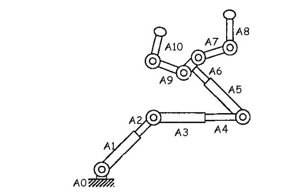
10 joint robot (Randomized Potential Fields Method).

In each of the above cases, the collision of the various links was explicitly checked in the same manner as the collision between the robot and the obstacles. Mechanical stops were imposed at each joints and the collision with each stop were also checked.

Bibliography

· Robot Motion Planning (Jean Claude Latombe) Kluwer Academic Press.

· Robot Analysis and Control (H. Asada, J. J. Slotine) John Wily and Sons.

· Manipulation Robots: Dynamics, Control and Optimization (Felix L. Chernousko, Nikolai N. Bolotnik, Valery G. Gradetsky) CRC Press.

· Mechanical Hands Illustrated (Ichiro Kato, Kuni Sadamoto) Survey Japan (1982).