Approximate Cell Decomposition

Index:

· Introduction

· General Description

· Approximate-and-Decompose

· Hierarchical Graph Searching

· Orientation Slicing

Introduction:

Here, we investigate another cell decomposition approach to path planning which is known as approximate cell decomposition approach. It consists again of representing the robot's free space C_free as a collection of cells. But it differs from the exact cell decomposition approach in that the cells are now required to have a simple prespecified shape i.e. rectangloid shape. As with the exact cell decomposition approach, a connectivity graph representing the adjacency relation among the cells is built and searched for the path.

        The time and space complexity of the methods based on this approach grows quickly with the dimension m of the configuration space. So these methods are good for small dimensions say m < 5.

General Description:

A rectangloid is closed region of following form in Cartesian Space Rⁿ:

{(x₁,x₂,….,x_n) | x₁Î [x₁′,x₁′′], x₂Î [x₂′,x₂′′],…, x_nÎ [x_n′,x_n′′]}

The differences x_i′′-x_i′ , i = 1,2,..,n are called the dimensions of the rectangloid.

Let W=cl(R). So,it is a rectangloid of R^m where m is the dimension of the configuration space C.

A rectangloid decomposition P of W (=cl(R)) is a finite collection of rectangloids {k_i}_i=1,..r such that:

· W = U k_i i=1,..,r

· "i_1, i₂ Î[1,r] i₁i₂ , int[] int[] = f

Each rectangloid k_i is called the a cell of the decomposition P of W.

Two cells are adjacent if and only if their intersection is a set of non-zero measure in R^n-1.

A cell K_i is classified as:

· Empty : if and only if its interior doesn’t intersect the C-obstacle region.

int (k_i) CB = f

· Full : if and only if k_i is entirely contained in the C-obstacle region.

k_i CB

· Mixed otherwise.

The connectivity graph associated with a decomposition P of W is the non-directed graph G defined as follows:

· The nodes of G are the empty and mixed cells of P.

· Two nodes are G are connected by a link if and only if the corresponding cells are adjacent.

Approximate-and-Decompose

This is a method for computing a rectangloid decomposition of a MIXED cell k. The goal of this method is to reduce the total volume of the newly created MIXED cells relative to the volume of k, while producing a reasonably small total number of cells.

For C = R²xS¹, the method can be applied as follows:

1.Outline
The approximate-and-decompose consists of first approximating the intersection of the CB with the cell k to be decomposed as a collection of non-overlapping rectangloids.
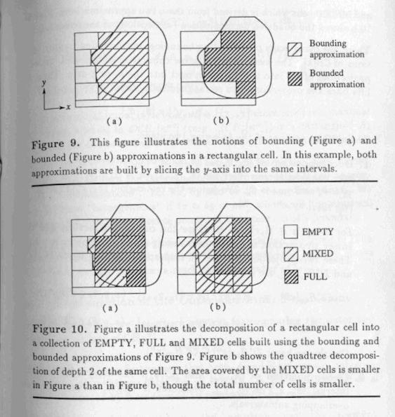
In order to generate EMPTY and FULL cells, as well as the MIXED cells, two types of approximations are computed: a bounding approximation and a bounded approximation.

Let CB(k) = CBk.

- A bounding rectangloid approximation of CB(k) is a collection of non-overlapping rectangloids R_i, i=1,..,p whose union contains CB(k).

o For every i[1,p] R_i k

o For every i, i' [1,p], ii¢ int(R_i)int(R_i¢) = f

o CB[k]

- A bounded rectangloid approximation of CB(k) is a collection of non-overlapping rectangloids R_i¢, i=1,..,p¢ whose union is contained in CB(k).

o For every i[1,p¢] R¢ k

o For every i, i' [1,p¢], ii¢ int(R_i¢)int(R_i¢¢) = f

o CB[k]

The EMPTY cells of the decomposition of k are obtained by computing the complement of in k.

The FULL cells of the decomposition are the Ri¢’s.

The MIXED cells are obtained by computing the complement of in every R_i.

The following figure illustrates the notion of bounding and bounded approximation.

Generating bounded and bounding approximations of CB[k]

Let k = [x_k,x′_k] [y_k,y′_k] [q_k,q′_k]

Then the method consists of the following two steps:

1. Decomposition of [q_k,q′_k] :

The range of orientations [q_k,q′_k] is cut into non-overlapping intervals [g_u,g_u+1], u = 1,..r, r > 0 with g₁=q_k and g_r+1=q′_k. Denote [x_k,x′_k] [y_k,y′_k] [g_u,g_u+1] by k^u.

For every u[1,r], we compute the outer projection and the inner projection of CB[k^u] into the xy-plane.

Outer projection, OCB_xy[k^u] = { (x,y)| q [g_u,g_u+1] : (x,y,q) CB[k^u] }

Inner projection, ICB_xy[k^u] = { (x,y)| q [g_u,g_u+1] : (x,y,q) CB[k^u] }

Clearly, ICB_xy[k^u] OCB_xy[k^u]

2. Decomposition of [x_k, x ′_k] and [y_k, y ′_k]:

For every u[1,r], the interval [x_k, x ′_k] or [y_k,y ′_k] whichever is longer is cut into non-overlapping subintervals.

Let us assume that [x_k, x ′_k] is subdivided. The general subintervals are [x_v, x _v+1], v=1,..,s, s > 0 with x₁ = x_k and x_s+1 = x ′_k. Denote [x_v,x_v+1] [y_k,y′_k] [g_u,g_u+1] by k^uv.

For every v[1,s], we compute the outer projection and the inner projection of OCB_xy[k^u] into the y-axis.

Outer projection, OCB_y[k^uv] = { y| x [x_u,x_u+1] : (x,y) OCB_xy[k^u] }

Inner projection, ICB_y[k^uv] = { y| x [x_u,x_u+1] : (x,y) ICB_xy[k^u] }

Clearly, ICB_y[k^uv] OCB_y[k^uv]

Each rectangloid [x_v,x_v+1] [c,c′] [g_u,g_u+1] where [c,c′] is a maximal connected interval in OCB_y[k^uv] (resp. ICB_y[k^uv]) is a rectagloid R_i (resp. R_i^¢) in the bounding (resp. bounded) approximation of CB[k].

Computation of Outer and Inner Projection of CB[k^u]

Principle: Let us first assume that both A and B are convex polygons and that A’s reference point lies in int(A). In R²x[0,2p], CB is a volume bounded by faces formed by patches of ruled surfaces.

Consider a point (x₀,y₀) in the xy-plane and the segment {(x₀,y_0,q) | q [g_u,g_u+1] } above this point. If the segment pierces a face of CB then (x₀,y₀) is in OCB_xy[k^u] but not in ICB_xy[k^u]. If it pierces no face, then either (x₀,y₀) is not in OCB_xy[k^u] or it is in ICB_xy[k^u]. The segment {(x₀,y_0,q)|q [g_u,g_u+1] } pierces a face F if and only if (x₀,y₀) lies in projection of F into the xy-plane.

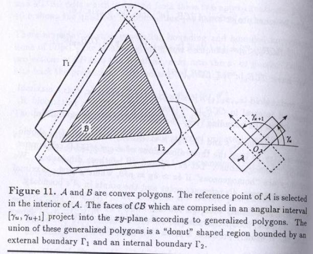
We show below that the intersection of every face with the interval [g_u,g_u+1] projects into the xy-plane according to a generalized polygon. Therefore, the projection of the boundary of CB that is comprised between g_u and g_u+1 is the union of generalized polygons. Under the assumptions made above, the union is a region with external boundary G₁ and internal boundary G₂. The generalized polygon bounded by G₁ is OCB_xy[k^u] and generalized polygon bounded by G₂ is ICB_xy[k^u].

The outer and inner projections of CB[k^u] are computed by:

1. Projecting all faces of CB (to the extent they are contained in the interval [g_u,g_u+1]) into the xy-plane.

2. tracking G₁and G₂ and clipping them by the rectangle [x_k,x_k¢] [y_k,y_k¢].

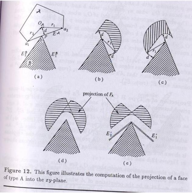
Projection of Type A face:

Let F_A be the face of type A comprised between limit orientations f₁ and f₂. The contact is between the edge E^A of A and vertex b of B.

The orientation f₁(resp. f₂) is achieved when the edge E^A is collinear with the edge E (resp. E).

Assuming that [f₁,f₂] [g_u,g_u+1], the projection is shown in the figure. It is obtained by the union of the two regions shown before.

The case where [g_u,g_u+1] [f₁,f₂] is treated in the same way after drawing two fictitious edges from vertex b.

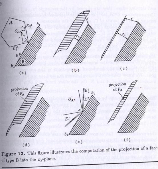
Projection of Type B face:

Let F_B be the face of type B comprised between limit orientations f₁ and f₂.

The contact is between the edge E^B of B and vertex a of A.

The orientation f₁(resp. f₂) is achieved when the edge E^B is collinear with the edge E (resp. E).

Assuming that [f₁,f₂] [g_u,g_u+1], the projection is shown in the figure. It is obtained by the union of the two regions shown before.

The case where [g_u,g_u+1] [f₁,f₂] is treated in the same way after drawing two fictitious edges from vertex a.

Computation of OCB_xy(k^u) and ICB_xy(k^u)

The contours G₁ and G₂ are computed by sweeping a line across the xy-plane. Assuming that [x_k,x_k¢] interval will be decomposed next in order to compute OCB_y(k^uv) and ICB_y(k^uv), the sweep line is chosen parallel to x-axis. The sweep starts from the smallest ordinate of all the points in the generalized polygons. During the sweep, the contours G₁ and G₂ are tracked by labeling the intervals comprised between the abscissae listed in the sweep line status as being outside OCB_y(k^uv), inside ICB_y(k^uv) but outside OCB_y(k^uv),or inside ICB_y(k^uv).

Once G₁ and G₂ have been extracted in the form of sequences of straight and circular edges, they are clipped by rectangle [x_k,x_k¢] [y_k,y_k¢].

Hierarchical Graph Searching

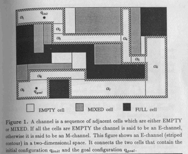
The first cut planning algorithm searches successive connectivity graphs G_i, i=1,2,.., until either it finds an channel of EMPTY cells connecting q_init to q_goal (success) or it doesn’t find any channel connecting these two configurations (failure ). Each graph G_i, i > 0 is obtained by from the previous one G_i-1, by decomposing the MIXED cells contained in the channel of MIXED cells found in G_i-1.

The major drawback of this algorithm is that the search work done in G_i-1 is not used to help the search G_i, although large subsets of these graphs may be identical.

Improved Algorithm:

The improved algorithm constructs a hierarchy of cg’s (connectivity graphs). The cg at the root corresponds to the first decomposition P₁ of W and we denote this cg by G^W. Every other cg in the hierarchy corresponds to the decomposition of the mixed cell k and denoted by G^k.

· Graph G^W is searched for a channel connecting q_init and q_goal. Assume that the outcome of the search is an M-channel P₁.

· Every mixed cell k in P₁ is recursively decomposed and searched for a channel that connects appropriately to the rest of P₁.

Once the M-channel P₁ been found out in G^W, P₂ is initialized to the empty sequence of cells and the planner consider every successive cell k in P₁ starting from the cell that contains q_init. If k is empty it is simply appended at the end of P₂ , if k is mixed it is decomposed into a set P^k of smaller cells. Let G^k be the cg associated with this decomposition. G^k is searched for a channel P^k that verifies following four conditions:

1. If k is the first cell in P_1,hence it contains q_init then the first cell in P^k also contains q_init.

2. If k is the last cell in P₁, hence it contains q_goal then the last cell in P^k also contains q_goal.

3. If k is not the first cell in P₁, the first cell of P^k is adjacent to the last cell of the current P_2.

4. If k is not the last cell in P₁, the last cell of P^k is adjacent to the cell following k in P₁.

P^k is called as subchannel.

If the planner succeeds to in generating P^k, P₂ is modified by appending P^k to it. The case when the planner fails, corresponds to the situation where the free space in the M-channel P₁ is disconnected by the C-obstacle region.

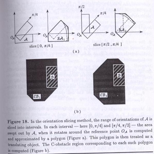
Orientation Slicing

This method consists of decomposing the range of the orientations of A into a finite number of intervals. In every interval, the area swept out by A as it rotates around its reference point O_A is computed and approximated by a polygon. This polygon is then considered as a translating object.

Let q_init = (x_init,y_init,q_init) and q_goal = (x_goal,y_goal,q_goal). The overall algorithm is as follows:

1. Decompose the range of orientations of A into a finite number of consecutive closed intervals [q_k,q_k¢] k=1,2,..p, such that q₁=0, q_k+1=q_k¢ (for all k Î [1,p-1]) and q_p¢= 2p.

2. For every k Î [1,p], compute the area swept out by A when it rotates around O_A from the orientation q=q_k to the orientation q=q_k¢. Approximate this area by a bounding polygon SA_k.

3. For every k Î [1,p], treat SA_k as the robot that is only allowed to translate with O_A as the reference point. Compute CB_k in SA_k configuration space C_k=R². Set C_k,free to C_k\CB_k.

4. For every k Î [1,p], decompose C_k,free into convex polygonal cells, using any method.( one is exact trapezoidal decomposition). Construct the cg G_k representing the adjacency relation between these cells.

5. Merge the graph G_k into a graph G by linking any two nodes X₁ÎG_k1, and X₂ÎG_k2, with k2 = k1+1 mod p, whenever the two cells corresponding to X₁ and X₂ intersect at a subset of non-zero area in R².

6. Search G for a path joining the initial cell to the goal cell. If the search terminates successfully, then return the sequence of cells along the path that has been found. Otherwise return failure.